Jacobians of Hyperelliptic Curves

TLDR. Hyperelliptic curves are really cool and doubly so because they can potentially generate groups of unknown order. But how do they work, and how do we determine how secure they are?

Introduction

In a recent IACR ePrint note 1, Samuel Dobson and Steven Galbraith proposed the use of the Jacobian group of a hyperelliptic curve of genus 3 as a candidate group of unknown order. The authors conjecture that at the same level of security, Jacobian groups of genus 3 hyperelliptic curves outperform the ideal or form class group in terms of both operational speed and representation size. Given the recent explosion of applications of groups of unknown order — verifiable delay functions, accumulators, trustless SNARKs, just to name a few — it is no wonder that this proposal was met with much enthusiasm. This note summarizes the mathematics involved in the hope to enable rapid deployment, but perhaps also to argue the case for caution.

For an engineer to deploy any group in practice, he must know:

  1. How to select public parameters for a target security level.
  2. How to represent group elements on a computer, and how to sample non-trivial group elements.
  3. How to apply the group law to pairs of group elements and, optionally, how to compute inverses.

This post summarizes the theory of hyperelliptic curves from an engineering point of view; that is to say, with an eye to answering these questions.

Divisors

Let $ \mathbb{F} $ be a field and $\mathbb{F}[x,y]$ the ring of polynomials in two variables. A curve is the set of points satisfying $0 = C(x,y) \in \mathbb{F}[x,y]$, along with the designated point $\infty$ called the point at infinity. While the coefficients of $C$ must belong to $\mathbb{F}$, when we consider the points satisfying the curve equation, we include points drawn from any extension field of $\mathbb{F}$. Let $\mathbf{C}$ denote this set of points. Such a curve is singular when for some point $P$, $C(P) = \frac{\partial{}C}{\partial{}x} (P) = \frac{\partial{}C}{\partial{} y} (P) = 0.$ (Just use the same old analytical rules for computing partial differentials; there is a finite field analogue for the definition of differentials that does not rely on infinitesimal quantities.) We need a non-singular curve $C$.

Let $\mathbb{E}$ be some finite extension of $\mathbb{F}$. The coordinate ring of $C$ over $\mathbb{E}$ is the quotient ring $K_C(\mathbb{E}) = \frac{\mathbb{E}[x,y]}{\langle C \rangle}$. The elements of this ring are polynomials in $x$ and $y$, but two such polynomials are considered equivalent if they differ by a multiple of $C$. Equivalently, $K_C(\mathbb{E})$ is the space of functions $\mathbb{E}^2 \rightarrow \mathbb{E}$ where we ignore the values the functions take in points not on the curve (so $\{P | C(P)=0\} \rightarrow \mathbb{E}$ would be a more precise signature). Furthermore, the function field $L_C$ is the fraction field of the coordinate ring of $C$, or phrased differently, $L_C(\mathbb{E})$ is the field whose elements are fractions with numerator and denominator both in $K_C(\mathbb{E})$.

Let $f(x,y)$ be a function in the coordinate ring $K_C(\mathbb{E})$. The order of vanishing of $f$ at a point $P$, denoted $\mathsf{ord}_f(P)$, is zero if $f(P) \neq 0$, and otherwise the greatest possible $r$ such that $f(x,y) = u(x,y)^r g(x,y)$ for some $g(x,y)$ with $g(P) \neq 0$ and for some uniformizer $u(x,y)$. The univariate analogue is when a polynomial $f(x)$ has a root of multiplicity $r$ at $P$, because in this case $f(x) = (x-P)^r g(x)$ for some $g(x)$ with $g(P) \neq 0$. Let $h(x,y)$ be a rational function from the function field of $L_C(\mathbb{E})$ of $C$, meaning that $h(x,y) = \frac{f(x,y)}{g(x,y)}$ for some $f(x,y), g(x,y) \in K_C(\mathbb{E})$. Then define the order of vanishing of $h$ in $P$ to be $\mathsf{ord}_h(P) = \mathsf{ord}_f(P) – \mathsf{ord}_g(P)$. When $f(P) = 0$, we refer to $P$ as a zero, and when $g(P) = 0$ it is a pole.

A divisor of $C$ is a formal sum of points, which is to say, we use the summation symbol but use the resulting expression as a standalone object without ever computing any additions. This formal sum assigns an integer weight to every point on the curve, and has a finite number of nonzero weights. Therefore, any divisor $D$ can be expressed as
$$ D = \sum_{P \in \mathbf{C}} c_P [P] \enspace ,$$ where all weights $c_P \in \mathbb{Z}$, and where the notation $[P]$ serves to identify the point $P$ and to indicate that it is not actually added to any other points.

Given two or more divisors, it is straightforward to compute their sum — just compute the pointwise sum of weights. This means that the set of divisors of $C$, denoted $\mathsf{Div}_C(\mathbb{E})$, is actually a group. Furthermore, define the degree of a divisor to be $\mathsf{deg}(D) = \sum_{P \in \mathbf{C}} c_P$. Then the set of divisors of degree zero is a subgroup: $\mathsf{Div}^0_C(\mathbb{E}) < \mathsf{Div}_C(\mathbb{E})$.

A principal divisor is a divisor $D$ that is determined by a rational function $h(x,y) = \frac{f(x,y)}{g(x,y)} \in L_C(\bar{\mathbb{F}})$, where $\bar{\mathbb{F}}$ is the field closure of $\mathbb{F}$, via
$$ D = \mathsf{div}(h) = \sum_{P \in \mathbf{C}} \mathsf{ord}_h(P) [P] \enspace .$$ Principal divisors always have degree zero. (This fact is rather counterintuitive. It is important to take the sum over all points in the field closure satisfying the curve equation, as well as the point at infinity.) Moreover, the set of principal divisors is denoted by $P_C(\bar{\mathbb{F}})$. It is a subgroup of $\mathsf{Div}_C^0(\bar{\mathbb{F}})$ and the restriction $P_C(\mathbb{E}) = P_C(\bar{\mathbb{F}}) \cap \mathsf{Div}_C^0(\mathbb{E})$ is a subgroup of $\mathsf{Div}_C^0(\mathbb{E})$.

We now have the tools to define the group we will be working with. The group of $\mathbb{E}$-rational points of the Jacobian of $C$ is $J_C(\mathbb{E}) = \frac{\mathsf{Div}_C^0(\mathbb{E})}{P_C(\mathbb{E})}$. Specifically, its elements are equivalence classes of divisors, with two members of the same class being considered equivalent if their difference is principal, or symbolically:
$$D_1 \sim D_2 \quad \Leftrightarrow$$
$$\exists f(x,y), g(x,y) \in K_C(\mathbb{E}) \, : \, D_1-D_2 = \sum_{P \in \mathbf{C}} (\mathsf{ord}_f(P) – \mathsf{ord}_g(P)) [P] \enspace .$$

Addition in this group corresponds to addition of divisors. However, there is no obvious way to choose the smallest (in terms of representation size) element from the resulting equivalence class when representing divisors as dictionaries mapping points to integers. For this we need to switch to a computationally useful representation of group elements.

Mumford Representation

The previous definitions hold for any generic curve $C$. Now we restrict attention to curves of the form $C(x,y) = f(x) – y^2$, where $f(x,y) \in \mathbb{F}[x]$ has degree $2g + 1$ and where $\mathbb{F}$ is a large prime field. This corresponds to a hyperelliptic curve and the number $g$ is referred to as the curve’s genus.

A divisor $D$ is called reduced if it satisfies all the following conditions:

  • It is of the form $\sum_{P \in \mathbf{C} \backslash \{ \infty \}} c_P([P] – [\infty])$.
  • All $c_P >= 0$.
  • Let $P = (x,y)$, then $y = 0$ implies $c_P \in \{0,1\}$.
  • Let $P = (x,y)$ and $\bar{P} = (x,-y)$ and $y \neq 0$, then either $c_P = 0$ or $c_{\bar{P}} = 0$ (or both).
  • $\sum_{P \in \mathbf{C} \backslash \{ \infty \}} c_P \leq g$.

There is exactly one reduced divisor in every equivalence class in $J_C$, and every reduced divisor corresponds to exactly one equivalence class in $J_C$. Therefore, we could have defined the Jacobian of $C$ to be the set of reduced divisors, except that the group law does not correspond with addition of divisors any more: the sum of two reduced divisors is not reduced. One could start from the addition rule for divisors and follow that up with a reduction procedure derived from the curve equation and the definition of principal divisors. However, it is by no means clear how this reduction procedure would work.

Mumford came up with a representation of reduced divisors that is conducive to finding the reduced representative of a divisor equivalence class. This representation consists of two polynomials, $U(x), V(x)$, such that all the following are satisfied.

  • $U(x)$ is monic.
  • $U(x)$ divides $f(x) – V(x)^2$.
  • $\mathsf{deg}(V(x)) < deg(U(x)) \leq g$.

The polynomial $U(x)$ is simply the polynomial whose roots are the $x$-coordinates of all finite points in the reduced divisor: $U(x) = \prod_{i=0}^{d-1}(x-x_i)$. The polynomial $V(x)$ interpolates between all finite points on the reduced divisor. It takes the value (or rather: one of two possible options) of the curve at all $x_i$. The divisor associated with $(U(x), V(x))$ is therefore $D = \sum_{i=0}^{d-1}([(x_i, V(x_i))] – [\infty])$. To find the Mumford representation of a divisor whose finite points are given by $\{P_i = (x_i, y_i)\}_{i=0}^{d-1}$, simply set $U(x)$ to the product as above, and determine $V(x)$ via Lagrange interpolation: $V(x) = \sum_{i=0}^{d-1}y_i \prod_{j \neq i} \frac{x-x_j}{x_i-x_j}$.

The cool thing about representing divisors as polynomials is their suitability for plots. Of course, to draw an elliptic or hyperelliptic curve we need to pretend that the field over which they are considered is continuous. However, many of the geometric intuitions drawn from continuous plots carry over to the discrete case.

Consider the elliptic curve $y^2 = x^3 -x + 1$, plotted below. Also plotted are the sets of intersection points of the lines $U(x) = 0$ and $y – V(x) = 0$ (dashed lines) for the following group elements presented here in Mumford representation:

  • $A: U(x) = x+1.2$ and $V(x) = 0.678$
  • $B: U(x) = x$ and $V(x) = 1$
  • $C: U(x) = x-1.27$ and $V(x) = -1.33$.

All these intersections do lie on the curve and therefore these polynomial pairs do represent valid group elements. The fact that $U(x)$ is linear and $V(x)$ is constant corresponds to the curve having genus 1, and also to the collapse of the set into just one intersection point for each group element. So we can use $A$, $B$, and $C$ simultaneously to denote the group element, as well as its representative as a point on the curve.

Let’s compute the group operation. The reduced divisor of the group element $A$ is $[A] – [\infty]$ and that of $B$ is $[B] – [\infty]$. Their divisor sum is $[A]+[B]-2[\infty]$. In order to find the reduced divisor from the same equivalence class, we must find a principal divisor that upon addition with this sum sends the two finite points to just one and decrements by one the weight of the point at infinity. Phrased differently, we must find a rational function $h(x,y) = f(x,y) / g(x,y)$ such that $[A] + [B] -2[\infty] + div(h) = [A+B] – [\infty]$, for some curve point which we denote with abusive additive notation as $A+B$.

The plot below shows one such option, plotting $f(x,y)$ in blue and $g(x,y)$ in red. Since $f$ and $g$ are themselves rational functions, their divisors must have degree zero. Indeed, $f$ has a pole of order 2 in $\infty$, and $g$ has a pole of order 3 there. Note that the finite intersection point between the red and blue lines does not appear in this formal sum of points: this absence corresponds with $g(x,y)$ and $1/f(x,y)$ having equal and opposite orders of vanishing in this point. The same phenomenon occurs at infinity, where $1/f(x,y)$ subtracts three from that point’s weight and $g(x,y)$ adds two back.

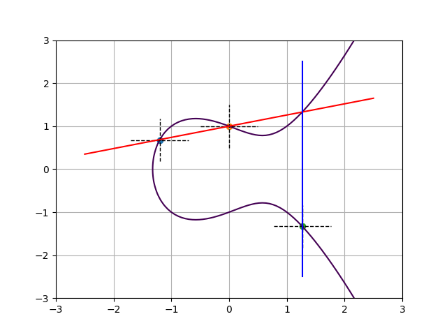
In other words, the chord-and-tangent rule for elliptic curves is just a special case of the Jacobian group law!

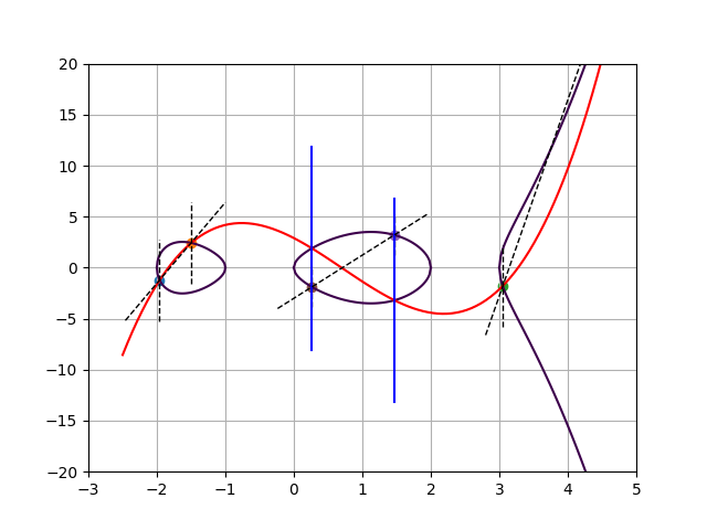
Let’s move on to a more complicated example. Below we have a plot of the genus 2 hyperelliptic curve $y^2 = x^5 -2x^4 -7x^3 +8x^2 + 12x$, with group elements $A$, $B$, and $C$ given by Mumford polynomials (dashed lines)

  • $A: U(x) = (x+1.96)(x+1.5)$ and $V(x) = 7.926x + 14.320$
  • $B: U(x) = (x-3.05)(x-5.03)$ and $V(x) = 19.204x – 60.383$
  • $C: U(x) = (x-1.467)(x-0.263)$ and $V(x) = 4.230x – 3.003$.

For each of these group elements, the lines $U(x) = 0$ and $V(x) = y$ intersect the curve in two points. In fact, this is a property of genus 2 curves, meaning that one can represent any group element by its two intersection points.

Since every group element corresponds to two elements on the curve, we have $\mathsf{div}(A) = [A_1] + [A_2] – 2[\infty]$, for the two points that represent $A$; and similarly for $\mathsf{div}(B)$ and $\mathsf{div}(C)$. To compute the group operation, we start from $\mathsf{div}(A) + \mathsf{div}(B) = [A_1] + [A_2] + [B_1] + [B_2] – 4[\infty]$ and search for a principal divisor $\mathsf{div}(h)$ such that sends the four finite points to two. One could start by finding the lowest degree univariate interpolating polynomial between the four points; this gives $f(x,y)$ which is plotted below in red. Note that $f(x,y)=0$ intersects the curve in six points $(A_1, A_2, B_1, B_2, \bar{C_1}, \bar{C_2})$, of which five are depicted in the plot. Furthermore, $f(x,y)$ has a pole of order 6 at infinity. Likewise, $g(x,y)$ intersects the curve in four points $(C1, C2, \bar{C1}, \bar{C2})$ and has a pole of order 4 at infinity. Therefore, the divisor equation
$$\mathsf{div}(A) + \mathsf{div}(B) – \mathsf{div}(C)$$
$$= [A1]+[A2]+[B1]+[B2]-4[\infty]-[C1]-[C2]+2[\infty]$$
$$= [A1]+[A2]+[B1]+[B2]+[\bar{C1}]+[\bar{C2}]-6[\infty]$$
$$-([C1]+[\bar{C1}]+[C2]+[\bar{C2}]-4[\infty])$$
$$=\mathsf{div}(f) – \mathsf{div}(g)$$ shows that as divisors, $A+B$ and $C$ are indeed apart by a principal divisor.

The two plots shown so far suggest a shortcut for representing group elements and computing the group operation thereon. Simply:

  • Represent group elements as points or sets of points on the curve.
  • When adding two group elements, fit a polynomial through all points and find the new points where it intersects the curve.
  • Flip the $y$-coordinates of these new points; this set is the new group element.

A natural question to ask is whether this intuition extends to curves of higher genus. That might be the case for all I know, but my intuition says “no”. Indeed, for curves of genus $\geq$ 3 no explicit point addition formulae are known and the preferred modus operandi for representing elements and operating on them is via their Mumford representations.

So how do we perform the group operation on Mumford pairs? That’s exactly what Cantor’s algorithm does. (Due to David Cantor and not Georg.)

Cantor’s Algorithm

Computes the composition of elements in the Jacobian group of the curve $y^2 = f(x)$.

  • Input: $(U1, V1), (U2, V2) \in (\mathbb{F}[x])^2$
  • Output: $(U, V) \in (\mathbb{F}[x])^2$
  1. Use the extended Euclidean algorithm to find the Bezout coefficients $h_1, h_2, h_3 \in \mathbb{F}[x]$ and $d \in \mathbb{F}[x]$ such that $d = \mathsf{gcd}(U_1, U_2, V_1 + V_2) = U_1h_1 + U_2h_2 + (V_1+V_2)h_3$.
  2. $V_0 \leftarrow (U_1V_2h_1 + U_2V_1h_2 + (V_1V_2 + f)h_3) / d$
  3. $U \leftarrow U_1U_2 / d^2$ and $V \leftarrow V_0 \, \mathsf{mod} \, U$
  4. $U’ \leftarrow (f-V^2)/U$ and $V’ \leftarrow -V \, \mathsf{mod} \, U’$
  5. $(U, V) \leftarrow (U’ / \mathsf{lc}(U’), V’)$
  6. If $\mathsf{deg}(U) > g$ go back to step 4
  7. Return $(U,V)$

The intuition behind the algorithm is that the polynomial $V_0$ is constructed to represent the divisor $\mathsf{div}(A) + \mathsf{div}(B)$. This polynomial is then reduced using the curve equation such that the degree decreases but the equivalence class remains the same. After reduction, the output is another Mumford pair.

Note that the polynomials considered all have coefficients drawn from $\mathbb{F}$, the plain old base field. This corresponds to restricting the Jacobian group to only elements defined over $\mathbb{F}$. Formally, let $\phi$ be the Frobenius map sending points $(x,y)$ to $(x^p,y^p)$ and $\infty$ to $\infty$, where $p$ is the order of the field $\mathbb{F}$. Then $\phi$ sends a divisor $D = \sum_{P \in \mathbf{C}} c_P [P]$ to $\phi(D) = \sum_{P \in \mathbf{C}} c_P [\phi(P)]$. A Jacobian group element (i.e., an equivalence class of divisors) is defined over $\mathbb{F}$ iff $\phi(D)-D$ is a principal divisor. In fact, by selecting the polynomials from the ring of polynomials over the base field, we guarantee that the Mumford pair determines a particular reduced divisor — the representative of its equivalence class — that remains unchanged under $\phi$. This implies that we can straightforwardly sample a non-trivial group element simply by sampling a Mumford representative; it is guaranteed to represent an element that is defined over $\mathbb{F}$.

Finally, the inverse of a group element $(U, V)$ is $(U, -V)$ and the identity is (1, 0).

Hyperelliptic Jacobians as Groups of Unknown Order

In the case of hyperelliptic Jacobians, the public parameters boil down to the curve equation and really, to the right hand side of $y^2 = f(x)$. Dobson and Galbraith recommend using an hyperelliptic curve of genus $g=3$, such that $f(x)$ has degree $2g+1=7$. Without loss of generality, $f(x)$ can be chosen to be monic, so there are only 7 coefficients left to determine. These should be drawn uniformly at random but such that $f(x)$ is irreducible.

The group is to be defined over a large enough prime field. In this case, an adaptation of Hasse’s theorem due to André Weil bounds the order of the group as

$$ (\sqrt{p}-1)^{2g} \leq #J_C(\mathbb{F}) \leq (\sqrt{p}+1)^{2g} \enspace .$$

Obviously we can’t determine the cardinality exactly because the whole point is that it should be unknown! However, the order must be sufficiently large because otherwise the discrete logarithm problem wouldn’t be hard.

The cheapest way to determine the order of the group is to determine the number points over $\mathbb{F}$ on the curve. For elliptic curves this can be accomplished using Schoof’s algorithm. There is an adaptation of this algorithm for genus 2 with complexity $O((\mathsf{log} \, p)^7)$. Dobson and Galbraith are unclear about what happens for genus 3, but another recent ePrint note 2 refers to work by Abelard for point counting in genus 3 curves that runs in $\tilde{O}((\mathsf{log} \, p)^{14})$ time.

Hyperelliptic curves of high genus admit index calculus attacks that are subexponential. For low genus $g \geq 3$, there is an attack in expected time $\tilde{O}(p^{2-2/g})$, which outperforms generic square root algorithms, whose complexity is $O(p^{g/2})$. For genus 2 curves the generic square root algorithms are faster.

There is a reduction due to Smith for translating the discrete logarithm problem on a genus 3 hyperelliptic curve to an elliptic one that works a sizable proportion of the time. After that translation, there is an algorithm due to Diem with estimated running time $O(p (\mathsf{log} \, p)^2)$.

The complexity of these attacks are plotted as a function of the number of bits of $p$ in the next figure.

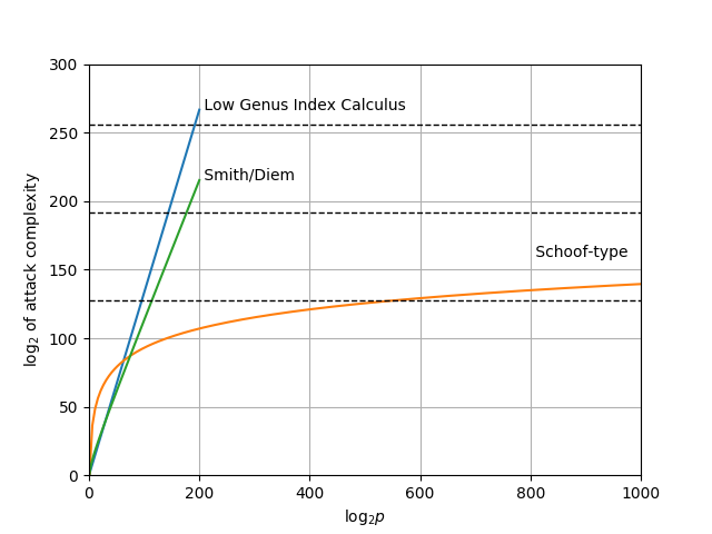
The orange line, which plots the complexity of the Schoof-type algorithm, is alarming. While it does cross the dotted line indicating 128 bit security (at $\mathsf{log}_2 \, p = 540$) it only crosses the 192 and 256 bit security lines for impractically large field sizes. The point of targeting 192 or 256 bits of security is not to hedge against improvements in the attacker’s computing power, because $2^{128}$ elementary operations is impossible within the lifetime of the universe according to our current understanding of its physical laws. Rather, the point of targeting $192$ or $256$ bits of security is to hedge against algorithmic improvements that cause the attack to require less computing work than anticipated. With respect to this objective, even a relatively minor improvement to the point counting algorithm would break the hedge as it decreases the actual security of conservative parameter choices by a large margin and massively increases the size of the base field required to provide the same target security level. In other words, it is not possible to err on the side of paranoia. Anyone looking to deploy genus 3 hyperelliptic curves for groups of unknown order must therefore be absolutely confident in their understanding of the best possible attack.

The exact complexity of point counting in curves of genus 3 remains a major open question with, until now, little practical relevance. However, as an alternative to understanding the complexity of point counting more exactly, it may be possible to generate groups of unknown order from similar mathematics but such that point counting does have the requisite complexity. For instance, we should not discount higher genera than 3, nor more generic abelian varieties.

Lastly, Dobson and Galbraith note that it is often easy to sample elements of small but known order. The capability to sample elements of known order violates the adaptive root assumption. The proposed solution is to instead use to the group $[s!] J_C(\mathbb{F}) = \{s! \, \mathbf{e} \, | \, \mathbf{e} \in J_C(\mathbb{F})\}$ for some large enough integer $s$ determined in the public parameters. This restriction kills off all elements of order up to $s$. When relying on the adaptive root assumption, for instance because Wesolowski’s proof of correct exponentiation is being used, it pays to represent the element $s! \, \mathbf{e}$ as $\mathbf{e}$, so that the verifier can verify that $s! \, \mathbf{e}$ is indeed a multiple of $s$ simply by performing the multiplication. Dobson and Galbraith argue that choosing $s = 60$ should guarantee a reasonable level of security, with $s = 70$ being the option of choice for paranoiacs.

To be honest, I am not sure I understand the argument by which the recommendation $s = 60$ is derived. It is something along the following lines. In Schoof’s algorithm (and derivatives) for point counting, an important step is to find points of order $\ell$. This translates to determining the order of the group modulo $\ell$, and via the Chinese Remainder Theorem the order of the group as an integer without modular reduction. Therefore, when we assume that determining the order of the group is hard, then there must be an $s$ such that constructing points of order $\ell > s$ is hard. The time complexity of this step of Schoof’s algorithm is $\tilde{O}(\ell^6 \mathsf{log} \, p)$ whereas the memory complexity is only $\tilde{O}(\ell^4 \mathsf{log}\, p)$, meaning that for large $\ell$, the running time will be the limiting factor. Extrapolating from implementation results reported on by Abelard in his thesis, setting $s = 60$ should be well beyond the capacity of an adversary running in a reasonable amount of time.

Personally, I prefer to draw the $\tilde{O}(\ell^6 \mathsf{log} \, p)$ complexity curve and set parameters depending on where it intersects with the target security level. The graph plotted below assumes $p \approx 2^{540}$ and pretends as though the polylogarithmic factor hidden by the $\tilde{O}$ notation is one. Note that the horizontal axis is the value of $\ell$ itself, and not its logarithm. For good measure I include the memory complexity (dashed orange line), in addition to the computational complexity (full blue).

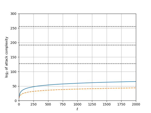
Based on this graph, I disagree with Dobson and Galbraith and recommend against using the Jacobian of a hyperelliptic curve for applications where the adaptive root assumption is supposed to be hard — unless with a solution that is different from restricting the group to $[s!] J_C(\mathbb{F})$.

Conclusion

Algebraic geometry, which is the field of mathematics that studies elliptic and hyperelliptic curves, is a powerful and versatile tool for generating cryptographic primitives. The recent proposal for generating groups of unknown order from hyperelliptic curves of genus 3, while exciting, is not without concerns. Specifically, a variant of Schoof’s point counting algorithm determines the group’s order in polynomial time, albeit a large degree polynomial. This complexity makes the selection of parameters to err on the side of safety nearly impossible and as a result, an accurate understanding of the best performing algorithm for this task is of paramount importance to anyone looking to deploy these groups in practice. Furthermore, the are algorithms that compute group elements with small but known order, violating the adaptive root assumption. These groups should not be used in constructions that require this assumption to hold, even if computing the order of the whole group is hard.

Nevertheless, the caution argued for in this article derives from a rather simplistic algorithm for determining the appropriate parameters: plot the computational complexity of the attack as a function of those parameters, and determine where that curve crosses the $2^{128}$ threshold. In reality, the attacker may require other resources as well — for instance, time, memory, parallel CPUs, or communication bandwidth between those CPUs. A more refined analysis may conclude that an assumed bound on the availability of these secondary resources will prohibit an attack long before it reaches $2^{128}$ elementary computational steps. Dobson and Galbraith are certainly not ignorant of the attacks on hyperelliptic curves nor of the standard simplistic methodology for deriving appropriate parameters. Therefore, I expect them to provide a more refined analysis in support of their proposal, perhaps based on other resource constraints. I will read that elaboration with much excitement when it appears.

Further Reading

  1. Samuel Dobson and Steven Galbraith: “Trustless Groups of Unknown Order with Hyperelliptic Curves” [IACR ePrint]
  2. Jonathan Lee: “The security of Groups of Unknown Order based on Jacobians of Hyperelliptic Curves” [IACR ePrint]
  3. Alfred J. Menezes and Ji-Hong Wu and Robert J. Zuccherato: “An elementary introduction to hyperelliptic curves” [link]
  4. Jasper Scholten and Frederik Vercauteren: “An Introduction to Elliptic and Hyperelliptic Curve Cryptography and the NTRU Cryptosystem” [link]
  5. Lawrence C. Washington: “Elliptic Curves: Number Theory and Cryptography, second edition” [home page]
  6. A straightforward implementation in Sage of hyperelliptic curves over prime fields [github repository]

On Nonlinear Noisy Key Agreement

TL;DR. A large number of post-quantum key encapsulation mechanisms (KEMs) and public key encryption schemes (PKEs) rely on noisy linear algebra problems. Interestingly, the addition of noise to make otherwise easy problems hard, is a strategy that remains restricted to linear algebra and fails to extend to nonlinear operations. This article explores why.

Noisy key agreement

Key agreement is a protocol by which Alice and Bob each send one message to the other and end up agreeing on a shared secret key. The eavesdropper Eve, who observes all messages in transit (but can’t modify them) remains incapable of computing this secret. The first such protocol was introduced by Diffie and Hellman and bears their names, but the general principle extends to generic algebras and not just commutative group theory.

For instance, let Alice and Bob agree on a common random integer G from a finite ring R, such as e.g. the set of nn matrices of integers modulo some prime p. Moreover, let Alice and Bob each sample their secret, a and b respectively, from this structure as well. They then exchange â = aG and b̂ = Gb, allowing both to agree on the shared key k = ab̂ = âb = aGb. Note that while the order of multiplication is important for matrices, by agreeing beforehand whose secret will be multiplied on which side of G, Alice and Bob circumvent this complication entirely.

Unfortunately, this protocol is completely insecure. Eve, who sees Alice and Bob agree on G before sending â = aG and b̂ = Gb, can compute G-1 and recover both Alice’s and Bob’s secrets, not to mention the shared secret key. Even if the ring disallows efficient computation of an element’s inverse, it remains extremely likely that there is a way to find the solution b to the system of linear equations Gb = b̂ and symmetrically for a.

The solution that makes the protocol a noisy key agreement protocol is to transmit only an approximation of aG and Gb. To see why this makes Eve’s task hard, observe how the error term 𝝐b = b̂ – Gb explodes: G-1b̂ = G-1(Gb + 𝝐b) = G-1Gb + G-1𝝐b = b + G-1𝝐b . Since G is a matrix with uniformly random coefficients, so is G-1 and multiplying that by another matrix 𝝐b — even if it has small coefficients — yields another random ring element that hides b much like a one-time pad.

However, the addition of small noise makes it difficult for Alice and Bob to agree on the same secret. Observe that Alice computes ka = a(Gb + 𝝐b) whereas Bob computes kb = (aG + 𝝐a)b. The trick is implied by the symbols’ case: instead of sampling uniformly random a and b, Alice and Bob sample a and b with small coefficients. If a, b, 𝝐a, and 𝝐b have small enough coefficients, then Alice’s view ka = aGb + a𝝐b is approximately the same as Bob’s view kb = aGb + 𝝐ab. As long as the difference a𝝐b – 𝝐ab is small enough, they can proceed to agree on an exact key with one additional message which either reconciles the two views or uses them in combination with error-correcting codes to transmit a wholly new message. In this last case, I like to refer the views ka and kb as shared noisy one-time pads or “snow-tipis”.

So how small should the secret elements a, b, 𝝐a, 𝝐b be? On the one hand, the secrets should not be too small because that reduces Eve’s search space. On the other hand, the secrets cannot be too large because then the difference a𝝐b – 𝝐ab is too large to enable either the reconciliation or transmission strategy. The situation is best described visually. While the unknown bits of the secrets do spread and multiply — and obscure Eve’s view — they also leave some bits of aGb intact; these bits can then be used as secret key material.

Incidentally, Ramstake, my own submission to the NIST PQC Project, does not quite follow this “intact bits” strategy of establishing common secret key material. Instead of having a few unknown bits at fixed locations, the secrets now have a few flipped bits at unknown locations. As long as the difference a𝝐b – 𝝐ab is not too dense, an error correcting code can help extract or transmit secret key material. Interpreting a darker shade of grey as representing a denser error distribution, this gives rise to the following analogous diagram.


Nonlinear Noisy Key Agreement

So why are there no nonlinear noisy key agreement protocols, or cryptosystems based thereon? Actually, that premise is not true. There is a submission to the NIST PQC project by the name of CFPKM whose underlying hard problem is polynomial system solving with noise (“PoSSoWN”). Alice and Bob compute their protocol contributions by evaluating a quadratic function f, which has small coefficients, in their secret vectors sa and sb, also with small coefficients, and by adding another small noise term. The underlying protocol is shown in the next figure. Unfortunately, despite the security proof, the cryptosystem was broken within weeks of the submissions’ publication.

The cryptanalysis exploits the observation that the keys computed by Alice and Bob differ only by the difference of element-wise products f(sa) ⨀ e2f(sb) ⨀ e1, which affects only the lower bits; whereas the high bits of both views are used for the session key. Importantly, these high bits are the same in b1b2, which is a value the passive adversary can compute as well.

So why is there no successful cryptosystem based on noisy nonlinear key agreement? The first observation is that the term nonlinear is really only relative to what the function’s arguments are. For instance, the expression x12 + 2x1x2x2 is nonlinear as a function of (x1, x2) but linear as a function of (x12, x1x2, x22, x1, x2, 1). By extending as we did here the vector of arguments of a function to a vector of all monomials occurring in that expression, any expression can be regarded as a linear function. In particular, both Alice’s and Bob’s computation of their proper views of the noisy secret key may be considered as linear transforms on some extended vector of monomials. This observation suggests a two-step approach to the diagrams above that indicate the source of secret key material: the second step captures the familiar linear noisy key agreement. The first step captures the extension of the original arguments into a vector of monomials.

This diagram highlights the origin of the problem: in order for there to be usable secret key material left at the end, the unknown bits in the extended vector of monomials must not be too many. In order for those unknown bits to not be too many, the unknown bits in the original arguments must be even fewer. However, this very salient feature makes these original arguments a vulnerable target for attack.

Conclusion

Why are there so few cryptosystems based on nonlinear noisy key agreement? My answer is twofold:

  1. Because any such protocol implies a linear noisy key agreement protocol.
  2. Adding nonlinearity to a linear noisy key agreement protocol makes it less secure.


Spooky Security at a Distance: The Controversy of Quantum Key Distribution*

*: An alternative title is obviously: Safe By The Bell.

TL;DR. Quantum cryptography offers the best of both worlds: security and quantum weirdness. In particular, quantum key distribution (QKD) is often claimed to offer “unconditional security based on the laws of physics”, a claim which is easily seen to be false. However, QKD does seem to be qualitatively more powerful than anything classical cryptosystems have to offer. This essay takes a critical look at the interplay between QKD and traditional cryptography by visiting the necessary background and summarizing the relevant concepts and context from a layman’s point of view.

1. Introduction

In the modern information age where computers are all around us, the need for computer security is greater than ever. It is no exaggeration to say that just about all our communication and financial infrastructure is protected by cryptography, the branch of computer security that deals specifically with protecting information. Calls to conduct government elections and identity management electronically should take their computer security requirements into careful consideration, or risk sacrificing national sovereignty and personal freedom to the whims of sufficiently sophisticated attackers — attackers who are sure to keep their algorithmic and technological advantages secret, thus making the estimation of security a very subtle game indeed.

Quantum technologies, i.e., devices that exploit quantum mechanical properties in a way that classical devices cannot mimic, are one recent development that is bound to dramatically affect the cryptographic landscape. While the end-goal of large-scale quantum computers is, despite significant resources devoted to the project, (presumably) not yet technologically feasible, detectors that measure the polarity of individual photons are already commercially available. Perhaps surprisingly, this on-going proliferation of quantum technology is causing a rift in the cryptographic community. On the one hand, the physicists are hailing the advent of photon detectors as enabling quantum key distribution and, by proxy, as the key to generating unconditional security — security beyond the traditional computational problems that are merely assumed, without proof, to be intractable. On the other hand, the mathematicians reject this notion of security guaranteed by physics; instead they prefer to stick to traditional computing hardware and design classical cryptographic algorithms to resist the end-game attacks by large-scale quantum computers.

Which side is right? The computer scientists, of course, because only they offer the proper computational perspective on the interplay between quantum mechanics and hard mathematical problems. More importantly, it is computer science and its parent, information theory, that offer the only rigorous definitions of security, namely in terms of confidentiality and authenticity. It makes sense then, to take a computer-scientific approach to assess the physicists’ and mathematicians’ claims. This essay does just that — it considers quantum key distribution from the point of view of theoretical computer science and cryptography by offering the layman reader an introduction to the subject matter and the necessary background. In the process we cover security-by-assumption; the strong Church-Turing hypothesis; quantum computation and entanglement; non-local-realism; Bell inequalities; and many more violations of common sense.

2. Cryptography

Cryptography is the science of protecting sensitive information against being read, modified, or otherwise used for nefarious purposes. While the use of cryptography dates back to the Ancient Greeks and beyond, the scientific investigation into this field of study is much newer, coinciding in large part with the information theory and computer science revolutions of the Twentieth Century. This coincidence is no accident as computers are experts at rapid information processing and are consequently the natural allies both of those who routinely generate and use sensitive information, but also — especially — of those who would attack its cryptographic safeguards.

2.1. One-Time Pad and Computational Security

One major result at the onset of this revolution is the proof by Claude Shannon — inventor of the eponymous information theory — that the one-time pad offers security against computationally unbounded adversaries1. Informally, by adding enough noise to a message, it becomes completely indecipherable to the eavesdropper, even though the intended receiver might be capable of reproducing the exact same stream of noise and thus recover the message. The label “unconditional security” is often applied when it is implicitly understood that the attacker fits the mathematical model and sees only the ciphertext in transit. By contrast, no such guarantee is offered against the attacker who violates this model by having access not only to the ciphertext in transit but also to another channel on the side — such as a watchful eye over the sender’s shoulder when the noise is added, or its equivalent in terms of a power consumption trace.

Unfortunately, unconditional security comes at the rather cumbersome cost of secret keys that must be at least as large as the message. Moreover, these keys must be distributed ahead of time, oblivious to the length of the message that is only chosen afterwards. In response, cryptographers have designed ciphers that mimic the one-time pad except for requiring only a relatively small key, independent of the message length. These ciphers do not offer unconditional security but computational security. That is to say, security only holds under an additional assumption to the effect that certain computational problems are hard to solve. This strategy of security by assumption may seem odd at first sight. However, considering that since the very successful standardization of the Belgian-designed AES algorithm2, the worldwide effort by cryptanalysts to break it have led essentially nowhere, it is fair to say that the entire computer security community is on board with this assumption. Moreover, any meaningful result on computational hardness would imply $\mathbf{P} \neq \mathbf{NP}$, the biggest unproven conjecture in all of computer science. This result would not only prove one of the seven millennium problems; it would also confirm mathematician’s suspicions that the other six are actually hard. Requiring a mathematical development of this magnitude seems like an unreasonably high bar for secure cryptosystems to pass.

2.2. Diffie-Hellman Key Establishment

Unfortunately, the shift towards computational security does not solve everything. Two parties wishing to communicate securely must still agree on a key beforehand, or else the eavesdropper will intercept the key and decrypt all subsequent traffic. Moreover, suppose $n$ parties wish to communicate; then there must be $n(n-1)$ shared keys for a complete graph. This strategy does not scale well.

A revolutionary solution to this problem was proposed by Diffie and Hellman in 19763, and for which they since won the Turing award. Their protocol, now called Diffie-Hellman key agreement, relies on the algebraic properties of groups as well as on the computational difficulty of computing discrete logarithms in them.

Consider for example $\left(\mathbb{Z}/p\mathbb{Z}\right)^*, \times$, the multiplicative group of integers modulo a large prime $p$. The discrete logarithm problem asks to compute $x$ from $g$ and $g^x \,\mathsf{mod}\, p$; there is no known efficient algorithm to perform this task on regular computers. Two parties, Alice and Bob, can use this group to establish a shared secret key by sending messages over an insecure channel; the eavesdropper cannot obtain this secret key.

The protocol proceeds as follows. First, Alice and Bob agree on a group element $g$ which will serve as the base number. Alice chooses a random integer $a \in \{0,…,p-1\}$ and sends $g^a \,\mathsf{mod}\, p$ to Bob; Bob mirrors this action by choosing a random integer $b \in \{0,…,p-1\}$ and sends $g^b \,\mathsf{mod}\,p$ to Alice. The group’s associative property guarantees that Alice and Bob can combine their own secret information with the message from the other to obtain a new group element $k=(g^a)^b=(g^b)^a \,\mathsf{mod}\,p$ which they use as the secret key for subsequent communication. On the other hand, the passive eavesdropper sees $g, g^a \,\mathsf{mod}\, p, g^b \,\mathsf{mod}\,p$ but this is not enough information to find $k$ efficiently. While there is no proof that obtaining $k$ from these values requires as much work as solving the discrete logarithm problem, in practice only groups are used in which this is widely believed to be the case.

Unfortunately, the Diffie-Hellman key agreement protocol only protects users from passive adversaries, i.e., adversaries who are content to only eavesdrop. By contrast, active adversaries who are capable of blocking messages and injecting them, are also capable of undermining the security of the protocol using a so-called man-in-the-middle attack. In short, the man-in-the-middle masquerades as Bob to establish a key with Alice; and masquerades as Alice to establish a key with Bob. Alice and Bob both think they have established a secret key with each other, but in reality they have both only established a secret key with the adversary. Any subsequent messages that are encrypted under one key are first decrypted by the adversary and then encrypted again under the other key before they are passed on.

The way security proofs get around this problem is by assuming it away. In particular, the authenticated links model explicitly states that the adversary is only passively observing and not blocking or modifying traffic4. The way this is solved in practice is by pre-distributing keys used for signature verification. Alice and Bob sign all their outgoing messages; they verify the authenticity of the incoming messages by verifying the attached signatures. The adversary cannot forge signatures on new messages because he is ignorant of the secret key. However, this solution requires that keys be distributed before communication begins, defeating the purpose of requiring no pre-shared information in the first place.

It is possible to separate signature verification from signature generation by requiring different keys for these operations. The private key, kept secret, is necessary for generating signatures, whereas the public key, broadcast to the world, is necessary for verifying them. The public keys themselves may be signed by yet other private keys and through a sequence of hierarchical hops reach a central authority. This strategy, called public key infrastructure, at least solves the scaling problem by requiring only a constant number of authority keys to be shared (as opposed to $O(n^2)$), although this solution comes at the cost of introducing a single point of failure.

2.3. The Quantum Revolution

Of course, any proposition about security that simultaneously reduces to computational hardness assumptions and claims to offer security in the real world, implicitly relies on a notion of computations that are physically realizable and at an acceptable cost. The first headway into answering this question was made by computer science pioneers Alonzo Church’s and Alan Turing’s formalizations of computation5 6 and the subsequent formulation of the Church-Turing hypothesis. Properly interpreted as a qualitative proposed law of nature, this hypothesis states that any process occurring in nature can be simulated by a Turing machine, a mathematical abstraction of what it means to compute due to Turing and inspired by Church’s lambda calculus. No physical experiments conducted thus far have indicated that the hypothesis as stated is false. Consequently, this has led computer scientists and physicists to pose a stronger version of this hypothesis, stating that all natural processes can be simulated efficiently 7 By contrast, this strong Church-Turing hypothesis seems to be — most emphatically — probably false.

In the 1990’s a series of results by pioneers in the field of quantum computation give strong evidence that quantum computers — computers that exploit the peculiar properties of quantum particles — are capable of solving some computational problems asymptotically more efficiently than classical computers. This string of results on quantum algorithms culminated in Shor’s celebrated work, which shows that the integer factorization and discrete logarithm problems, while difficult on classical computers, are in fact easy on quantum computers8. Not only is Shor’s algorithm strong evidence that the strong Church-Turing hypothesis is false; it is also practically relevant as it breaks the security of the Diffie-Hellman protocol described above. The situation is even worse: switching to RSA or to elliptic curve cryptography (ECC) will not help as RSA crucially relies on the difficulty of the integer factorization problem and elliptic curve cryptography on the general formulation of the discrete logarithm problem — both of which are still susceptible to Shor’s attack. In fact, in the foreseeable future when large-scale quantum computers exist, most public-key cryptography widely deployed today will become insecure. More importantly, information encrypted today can be stored for the future at very low cost until a point at which quantum computers do exist; from this point of view, Diffie-Hellman, RSA and ECC are already insecure.

In response to this threat, researchers are designing and developing post-quantum cryptosystems — cryptographic algorithms that can be executed on traditional computers but promise to offer security even against quantum computers9. The way these cryptosystems accomplish this feat is by reducing their security properties to other computational hardness assumptions, notably different from the integer factorization and discrete logarithm problems and hence very arguably immune to Shor’s attack. While the selection of post-quantum cryptosystems is large enough to sustain a scientific discipline in and of itself, they suffer from two significant disadvantages. One, they are inefficient in one way or another: either the public key, message size, or computational requirements are rather large, thus making their adoption an unattractive course of action. Two, they rely on relatively under-studied cryptographic hardness assumptions; anyone who uses a post-quantum cryptosystem over RSA or ECC is consequently making a larger gamble with respect to security. Nevertheless, in some cases such as hash-based signatures, the security can be reduced to assumptions which are already commonplace; cryptographic assumptions so minimalistic that if they turn out to be false, no computationally-secure cryptography whatsoever would be possible in the first place.

3. Quantumness

Quantum particles behave in undeniably peculiar ways. For instance, the complete description of a system of $n$ qubits — i.e., $n$ independent binary properties of quantum particles — requires a vector of $2^n$ complex numbers with Euclidean length one; we refer to this vector as the system’s state and denote it using Dirac ket notation: $|a\rangle$. By contrast, the complete description of n classical binary variables requires $n$ bits. In this sense, a quantum system is much more akin to a probability distribution over strings of $n$ bits; a complete description of such a probability distribution requires $2^n$ real numbers between zero and one and whose sum is one (as opposed to its sum-of-squares).

This comparison of quantum states to probability distributions is no accident. Every quantum state associates a complex-valued amplitude to each observable event. By squaring the modulus of this number, one obtains the probability of measuring this outcome. However, upon employing measurement, the quantum state collapses; it assumes amplitude one in the component associated with the observed event and amplitude zero in all other components. While this sounds familiar to sampling classical probability distributions, the surprising fact is that quantum states exist — it is possible to define and perform experiments whose observations cannot be explained without recourse to this exponentially-large complex-valued state vector. By contrast, classical probability distributions are merely a method invented by humans to cope with hidden variables that do have a definite but unknown value.

In the terminology of quantum physicists and quantum computer scientists, an impure quantum state constitutes a superposition of values. Moreover, by manipulating the particles used to represent these qubits it is possible to generate constructive or destructive interference i.e., cause the amplitudes add or cancel out. Moreover, it is possible to generate quantum states where measuring one particle only partially collapses the state, because the other particles still remain unmeasured. This phenomenon is known as entanglement and has generated much controversy in the past.

3.1. The EPR Paradox and the Bell Inequality

Entanglement means that measuring one particle can influence the probability distribution associated with measuring another particle. In other words, one cannot reason meaningfully about counterfactual observations because the world in which the experiment is performed is fundamentally different from the world in which it isn’t. If this idea makes you uncomfortable, you are in good company. Albert Einstein famously rejected this notion, insisting that Nature had to follow the principle of realism: reality does not change depending on whether you observe it or not. Phrased differently, the moon does not pop into existence the second you decide to look at it.

Together with co-authors Podolsky and Rosen, Einstein formulated a seemingly devastating blow to the theory of quantum mechanics10. The EPR thought experiment takes two entangled particles and separates them in space by a large enough distance. Then quantum mechanics predicts that the act of measuring one particle will exert an influence on the other particle, as borne out by a different probability distribution associated with measuring it, faster than the speed of causality. While Einstein understood that this principle could not be used to transmit information — thus not violating the second fundamental postulate of special (and general) relativity outright — this sense of influence-faster-than-causality certainly violates the spirit of relativity, and gave rise to the fantastically playable phrase “spooky action at a distance”.

The EPR paradox subtly sneaks in a second assumption about Nature, in addition to that of realism. In order for this “spooky action” to have to travel in the first place, the information describing one particle’s state, before and after measurement, has to be localized — independent of other events elsewhere. Phrased differently, the moon exists whether or not the sun is shining. This principle of locality, in conjunction with its brother realism, is known as local-realism; the contradiction predicted by quantum mechanics is known as non-local-realism.

Twenty-nine years after the publication of the EPR paradox, a physicist by the name of John Stewart Bell showed that local realism is not just a philosophical ponderance; it is a falsifiable hypothesis about nature11. In other words, it is possible to perform experiments whose measurement results will indicate whether we live in a local-realist world or not. The intuition is as follows. If Einstein’s conception of quantum mechanics is correct, then there exists information hidden inside a quantum system that determines the measurement outcome. By preparing the system in a controlled manner, this hidden information is guaranteed to follow a probability distribution, and by performing the experiment many times the observed variables are guaranteed to follow that probability distribution, even if these observables measure in large part the same property.

By contrast, quantum mechanics precludes any such probability distribution where the same property can be independently sampled by two different observables. The first measurement will influence the state and the second measurement measures a different state, hence giving rise to other borne probabilities. Unfortunately, this state collapse makes the system look as though it was behaving conformant to local-realism the entire time and any measurement following the collapse cannot decisively indicate non-local-realism. Bell’s crucial insight was that the world-distinguishing information is not located in individual measurement variables, but rather their correlation, or more generally, their mutual relations.

Consider this excellent example due to Sakurai12, of a quantum system consisting of two perfectly entangled photons having an unknown but equal polarization. The photons are sent to Alice and Bob, at opposite ends of the universe. Their polarizations are measured along one of three axes, $x$, $y$ and $z$, each $120^\circ$ apart and in the plane but such Alice’s set of axes coincides with Bob’s. Obviously, if they choose to measure along the same axis, they are guaranteed to obtain the same result, 1 (the photon detector fires) or 0 (no activity is registered).

If it is true that the photons’ polarization is completely fixed and independent of the measurement at either end of the universe, then whatever preparation device that produces the photons follows a probability distribution $p(x,y,z)$ describing the probability of observing the photon at any of the three axes. Being a probability distribution, the sum over all events of that event’s probability equals one:

$$ \sum_{x \in \{0,1\}} \sum_{y \in \{0,1\}} \sum_{z \in \{0,1\}} p(x,y,z) = 1 \enspace .$$

Moreover, Alice and Bob’s measurements don’t influence the state of the quantum system; they merely obtain information about it. Consequently, their joint statistics may be used to qualify this probability distribution, for example in the following way.

$$ {\rm Pr}[x=y] = p(0,0,0) + p(0,0,1) + p(1,1,0) + p(1,1,1) $$
$$ {\rm Pr}[x=z] = p(0,0,0) + p(0,1,0) + p(1,0,1) + p(1,1,1) $$
$$ {\rm Pr}[y=z] = p(0,0,0) + p(1,0,0) + p(0,1,1) + p(1,1,1) $$

The sum of the probabilities of these non-mutually-exclusive events must thus satisfy $$ {\rm Pr}[x=y] + {\rm Pr}[x=z] + {\rm Pr}[y=z] = 1 + 2p(0,0,0) + 2p(1,1,1) \geq 1 \enspace . $$

In the intuitive words of Preskill, “whenever three coins are on the table, and each one is either an H or a T, then at least two of the three have to be the same”13. However, Alice and Bob experimentally confirm that ${\rm Pr}[x=y] = {\rm Pr}[x=z] = {\rm Pr}[y=z] = (\mathsf{cos} \, 120^\circ)^2 = 0.25$ and hence

$$ {\rm Pr}[x=y] + {\rm Pr}[x=z] + {\rm Pr}[y=z] < 1 \enspace , $$
thus violating the Bell inequality.

In practice, experiments prefer to use the less accessible CHSH inequality14. However, the same principle is used: EPR local-realism and quantum entanglement predict different measurement statistics. Since Bell’s original 1964 paper, there have been many variants of his equation and even more experimental validations — that is to say: violations of the inequality — deciding in favor of the non-local-realism of quantum mechanics beyond reasonable doubt.

3.2. Quantum Key Distribution

So if we can’t observe particles without disturbing them, how about using this to our advantage? Specifically: certain actions are quantum mechanically impossible; can we put these impossible tasks on the only path between the attacker and our sensitive information, in the same sense that computationally infeasible tasks block this path now? The answer is yes, it is possible to use quantum mechanics to protect information. It turns out entanglement isn’t even required.

In 1984, two researchers by the name of Bennet and Brassard proposed what is now known as the BB84 protocol: a mechanism for key distribution relying on the polarization of photons15. Alice chooses a string of bits from which to derive the key. She then sends a string of individual photons where each bit of her secret bit string is encoded in the photons’ polarization, with respect to rectilinear ($+$) or diagonal ($\times$) bases as determined by random coin tosses. Bob measures the incoming photons with respect to rectilinear or diagonal bases as determined by his own random coin tosses. Whenever Bob chooses the same basis as Alice, there is a small probability of the photon not being measured at all, but if it is measured it is guaranteed to produce the same bit Alice sent. On the other hand, if the photon is measured in opposite bases, Bob’s measured bit will be uniformly random.

After measuring the photons with respect to random bases, Bob announces these chosen bases to Alice over a public classical channel, along with an indication which bits were actually received. Alice responds by identifying which choices of basis were correct, thus indicating which of Bob’s measured bits are identical to Alice’s. A few of these correct bits are also exchanged just to guarantee with high probability that there is no eavesdropper on the quantum channel.

Security is guaranteed by the following rationale. Suppose an eavesdropper named Eve is observing the photons on the quantum channel with respect to her randomly chosen bases. And suppose she sends out new photons towards Bob with the polarization that she measures. Then whenever Alice and Bob used the same basis, there is a $1/2$ chance that Eve’s basis is opposite. If this is the case, Bob’s measurement will be the same as Alice’s with probability $1/2$. So by exchanging $k$ agreed upon bits in the last step, Alice and Bob reduce the probability of a successful eavesdropper to $(3/4)^k$. Table 1 is drawn straight from BB84’s paper and summarizes the steps involved.

Table 1. The BB84 protocol in action.

In 1991, a couple of years after the BB84 protocol, Artur Ekert proposed another construction for key distribution based on quantum entanglement16. While Ekert’s protocol is rather more difficult to realize physically, the security guarantees it offers are vastly different from the ones offered by the BB84 protocol, so it is certainly worthwhile to take both protocols into account.

In Ekert’s protocol, the quantum channel consists of a source of pairs of entangled particles sent to opposite ends of the channel. The emitted particles are in the singlet state: $|S\rangle = 1/\sqrt{2} |\uparrow\downarrow\rangle – 1/\sqrt{2} |\downarrow\uparrow\rangle$, guaranteeing that whatever spin is measured at one end, the other end must measure the opposite spin provided the same basis is used.

Both Alice and Bob measure the particles headed their way in random bases. After this measurement, they communicate over a public classical channel to determine in which cases both Alice and Bob registered a measurement in the same basis. At this point, they release the measurements obtained when their measurement bases were unequal; this allows them to determine statistical variables for which the CHSH inequality (an inequality of the Bell family) should be violated if the particles are properly entangled.

An eavesdropper who measures the particles’ spin in random bases just before the particle reaches Bob and then sends out a new particle with the measured spin, cannot violate the Bell inequality. Consequently, this eavesdropper will be detected with very high probability.

The reliance on Bell’s inequality removes the requirement to trust the device that produces the quantum particles to be honest: malicious devices cannot pass the Bell test. Consequently, this type of quantum key distribution is called device-independent.

3.3. Authentication

At this point we have glossed over a key assumption on the adversary: he can look, but not touch. In other words, the adversary is assumed to be somewhat passive. While he is allowed to read messages, his cannot block, modify, or create them.

Of course, in a realistic scenario, the adversary is capable of active intervention. In this case, he can perform the man-in-the-middle attack: impersonate Bob in the eyes of Alice, and impersonate Alice in the eyes of Bob. Both Alice and Bob think they’re establishing a secure connection to the other, but in reality they are only establishing a secure connection to Eve, the (wo)man-in-the-middle. Even the Bell test cannot help because at most it will indicate that Alice’s connection to Eve and Bob’s connection to Eve were both generated using properly entangled particles.

In practice, the only way to block a man-in-the-middle attack is to authenticate the messages that are sent over the public classical channel. This variant of digital signatures allows the receiver, who knows the secret key, to verify beyond doubt that the messages were sent by the other owner of the secret secret key and that the messages were not modified in transit. Under the assumption that the adversary does not know this secret key, an authentication scheme thus offers two properties: entity authentication, the sender is who they say they are; and data integrity authentication, the data has not been tampered with. Unfortunately, any secure authentication scheme requires a pre-shared secret key, thus cancelling in large part the very point of quantum key distribution in the first place. Moreover, the authentication schemes used in practice, for example in internet protocols such as TLS, rely once again on hard problems to guarantee security. But the whole point of QKD was to not have to rely on computational problems at all!

Fortunately, though, the outlook for quantum key distribution is not quite as bleak. There exist unconditionally secure authentication schemes whose security does not rely on the intractability of computational problems, such as the Wegman-Carter scheme17. The reason they are not used in TLS, for example, is because they consume secret key material as they are used, in the same sense that the one-time pad consumes secret key material as it is used. Use the same secret bits twice and the security of the scheme is broken. However, in the case of authentication and in contrast to encryption, the length of the secret key can be shorter than the processed data. This means that it is possible to use a short shared secret key to authenticate quantum key distribution which then generates a longer shared secret key. From this point of view, the term quantum key distribution is a misnomer; it should be quantum key-length extension.

4. Criticisms of QKD

Quantum key distribution can obviously offer security properties that classical cryptography is incapable of offering. So why is the reception of quantum cryptography lukewarm at best among traditional cryptographers? We explore several possible reasons.

4.1. Implementation Issues

Quantum key distribution is not just an idea; it is supposed to be implemented in practice using physical matter. Consequently, it might be very difficult or even impossible to engineer this physical matter into behaving according to the protocol. Conversely, the adversary against which the protocol is supposed to protect might have access to the physical device through side-channels that the security model does not account for.

The possibility of side-channel attacks was observed in the very first practical demonstration of the BB84 protocol, which the authors describe as being “unconditionally secure against any eavesdropper who happened to be deaf! :-)”18. Indeed, the listening adversary could hear the polarization filters rotating and would be able to infer the chosen bases from the sound. Another example considers the difficulty of generating a laser pulse containing exactly one photon. But if the pulse contains multiple photons, the adversary can get away with measuring the polarity of one of the superfluous ones, leaving the one photon that travels all the way to Bob intact. A final example considers an implementation attempting to get around the rotating filters problem by generating photons of different polarization by different sources. Unfortunately, this implementation does not take into account that different sources have a unique spectral signature, which grants the adversary access to another side channel leaking information on the chosen bases. An excellent survey of practical issues is due to Scarani and Kurtsiefer19.

It is clear that requiring specialized hardware for instantiating quantum key distribution protocols generates its own set of specific problems, each one requiring significant engineering considerations to circumvent. By contrast, traditional cryptography is by design implementable on standard computer hardware. The all-too-common pitch that quantum key distribution offers “security guaranteed by the laws of physics” is clearly false if the adversary has side-channel access to the QKD devices. Likewise, the security of traditional cryptographic algorithms breaks down whenever the attacker has side-channel access to the computing device — but in this case at least the notion of “side-channel access” is well-defined and empirically bounded: power consumption, timing information, acoustic and electromagnetic wave emanation, voltage of probed wires … and that’s about it. In order to instantiate secure quantum key distribution, one has to take into account many more, vastly different, and unpredictable side-channel attacks.

4.2. Quantum Eavesdropper

It is tempting to compare the adversary in the quantum key distribution protocols with the passive adversary in classical key distribution protocols. However, this comparison does not quite hold. The passive adversary in classical cryptographic protocols is allowed to observe data in passing; he is merely not allowed to modify. By contrast, in the quantum case observing is modifying; by making observation and modification inseparable, quantum key distribution is introducing a model that is simultaneously weaker and stronger than the passive model of classical protocols, albeit for good reason (i.e., the laws of physics).

Except, observation is equated to measurement, which necessarily collapses the state. However, especially in the realm of quantum phenomena there exist manipulations which are more subtle than measurement but nevertheless akin to observation. In particular, consider the quantum computer20 that, having access to its own, secret qubit prepared in the state $|s\rangle = |0\rangle$ manipulates the photon heading to Bob by performing the computation $|b,s\rangle \mapsto |b,s\oplus{}b\rangle$. This quantum operation is unitary and does not violate the no-cloning theorem because after the computation is done the eavesdropper’s qubit is not independent of the passing photon; by contrast, it is perfectly entangled with it. Once Bob makes known the bases in which he measured, then the quantum computer uses the same basis to measure its secret qubit, thus obtaining the exact same bit Bob obtained.

Ekert’s protocol implicitly deals with this attack as it is a subcase of the explicitly considered situation in which three entangled particles rather than two are emitted by the source. Bell’s inequality comes to the rescue: the statistical test cannot be satisfied if three particles are entangled rather than two. In other words, not only can the Bell test distinguish between some entanglement and no entanglement; it can also distinguish between some entanglement and even more entanglement. While the adversary can get away with eavesdropping on a few particles in this manner, the probability of this misbehavior being noticed rises with the number of ‘observed’ particles. This is precisely the reason why quantum key distribution protocols are often enhanced with another “privacy amplification” step, in which the string of shared secret bits of which the adversary might know some individual bits is transformed into a bitstring of which the adversary does not know any individual bits but instead some minimal amount of general information.

However, the BB84 protocol is vulnerable to this attack precisely because there is no Bell test. More importantly, there cannot be a Bell test in the BB84 protocol because there is no entanglement; there is no “third coin” whose non-existence must be indicated by the statistical information. Phrased differently, there is no counterfactual event whose occurrence would have caused different observations. The measurement statistics in this protocol conform to local realism.

However, it is not clear that even if quantum computers can be built that they should also be capable of intercepting photons, computing on the qubit represented by its polarization, and send out a photon with a polarization matching a given qubit. Nevertheless, this possibility is implied by the conjectured possibility of quantum routers and relays that enable quantum key distribution across many hops and storing them in quantum memory for a little while at each point. Moreover, the alarming fact is that this attack is not ruled out by quantum physics. Quantum key distribution is, after all, one of the proposed solutions to the threat of quantum computers and their break of widely deployed public key infrastructure. It would seem that the claims of security against quantum computers are restricted only to device-independent QKD.

4.3. Nothing Wrong with Computational Security

Perhaps most fundamentally, the chief selling point of quantum key distribution attests to a deep-seated distrust in computational hardness assumptions — a distrust that cryptographers, in general, are unlikely to share. It is fairly reasonable to assume that the discrete logarithm and integer factorization problems may one day be easy; Shor’s algorithm predicts as much. However, it is another thing altogether to conjecture that AES will one day be easy to break or that collisions to SHA2-256 will one day be found. Cryptographers will not take the people who make these claims seriously unless they are preceded by breakthrough results. However, anyone who prefers the clearly-not-unconditional security of quantum key distribution over the merely-computational security offered by AES or SHA2 is implicitly making exactly these claims. QKD proponents who don’t want to make these claims even implicitly must consequently argue for quantum key-length extension until the shared key reaches 256 bits, after which point computational cryptography over the classical channel is perfectly adequate. But in this case the usefulness of QKD is restricted to the world in which it is feasible to establish shared and perfectly secret strings of less than 256 bits but for some reason it is not feasible to do the same for a string of 256 bits or longer.

Nevertheless, there is eminent justification for skepticism regarding the conjectured computational difficulty of the problems underlying post-quantum cryptosystems for public key encryption and Diffie-Hellman key agreement. These problems are after all new and under-studied, and don’t secure large monetary rewards for whoever solves them. However, perhaps one day, after resisting many years of attempted cryptanalysis and being duly recognized by national and international standardization bodies, a subset of these problems can achieve the same status as AES and SHA2 — and inspire the same confidence. Indeed, not only is this likely to happen, it is the desirable outcome. At that point, the same criticism applies to quantum key distribution: what advantage does it offer over a classical cryptosystem relying on hard problems that are trusted anyway?

5. Conclusion

Quantum physics speaks to the imagination because it is so viciously counter-intuitive. It rejects many rules of thumb that make perfect sense in the macro world, such as counterfactual events having well-determined outcomes; or such as information having to travel in order for one event to exert influence on another. It is all too easy to ascribe some mystical properties to the workings of quantum mechanics because to the uninitiated it truly is indistinguishable from magic.

To a lesser degree, the field of cryptography is also familiar with this mysticism. Cryptography deals with problems that are difficult by design — they must be, because otherwise they would be ineffective. In the eyes of popular science it takes many years of studying complex mathematical formulas before being able to grasp this spirit of difficulty.

It is perfectly understandable then, that the combination quantum + cryptography speaks to the imagination beyond what either branch is capable of by itself. It is a self-selling sales pitch that lodges itself firmly in the pitchee’s mind in that special place allocated for whatever thought is capable of producing a sense of wonderment about the world. No doubt this enticing nature has helped secure funding on the topic for many years to come.

Except, that’s not how science works. It is wrong and unscientific to worship the priests for informing us about the truth. It is a disservice to all three fields — quantum information theory, cryptography, and the overlap — to ascribe importance to the technology of quantum key distribution due to its perceived mystical properties. The researchers in these fields hold themselves to the highest (and most definitely anti-mystical) standards of verifiability and reproducibility and to pretend otherwise is to level an insult. Either quantum key distribution produces material benefits or it does not, and the quality of this invention should be assessed accordingly.

Without a doubt, we have seen that quantum key distribution is capable of offering security properties that no classical cryptosystem can offer. However, the setting in which these special security properties become relevant is rather artificial and constrained. By contrast, the promulgation of quantum key distribution technologies seems to focus on the BB84 variant, which introduces a whole host of new security hazards, to the point where the claimed security “benefit” is very dubious indeed.

In the end, it will not be the theoretical computer scientist who decides which technologies are useful and which are not — nor should it be. It will instead be the engineer who plots graphically the implementation cost on one axis against the security requirements on the other, and comes to a conclusion based on considering the relative positions of all competing options. Quantum key distribution may well occupy a location on this graph that justifies its existence. But until quantum key distribution proponents take the existence of this cost-benefit-graph into account and pinpoint QKD’s location on it, QKD is bound to remain only a theoretical exercise with the occasional proof of concept supporting its physical possibility.